Viterbi, my favorite algorithm

published 2013-03-03 [ home ]

The State Machine

Let us consider a system that can take a finite number of states S[1] to S[n] over time.

We can represent the system as a N-node directed graph, where nodes are the states. An arc exists between node S[i] and S[j] if the system can transition from S[i] to S[j]. You probably already know that.

In Chains

We will now observe the evolution of the system over time. We will model time discretely. That does not mean that time itself is discrete, but we will observe the system at fixed-interval “ticks”. We call S(t) the state of the system at tick t.

If the system is known to be in S[i] at tick t (i.e. S(t) = S[i]) we call P(i->j) the probability that it will be in S[j] at tick t+1. Here is a definition for the mathematically inclined: P(i->j) = P(S(t+1) = S[j] | S(t) = S[i]).

A few remarks:

P(i->j) is considered independent of t;
P(i->i) exists;
the sum of outbound probabilities is 1: ∀i, ∑[j=1,N]{P(i->j)} = 1.

By the way, this is called a Markov Chain.

Blurry Sights

Now let’s complicate things a little by introducing a separate system that can take states V[1] to V[M]. This second system V is tied to S: at every tick t, the probability distribution of V(t) only depends on S(t). We will note: O(i,j) = P(V[j] | S[i]).

You can think of V as something that observes S and reports on its state in an incomplete and probabilistic manner.

If you have understood everything up to now, you should easily get what this means: ∀i, ∑[j=1,M]{O(i,j)} = 1.

If you have not, let’s take a really simple example with N = M = 2. You can imagine that both S and V are lights that can be either red or blue. The relationship between S and V can be expressed by something like this: “If light S is red, then there is 90% chance that V is red too. If light S is blue, then there is only 40% chance that V is red.”

Now, add more possible colors to S and V, not necessarily the same number for both, to generalize the system.

The Black Box

Now, here is our problem: imagine that you know how system S works (the probabilities of transition between the states) but that it is hidden in a black box such that you cannot observe it. What you can observe is system V. Is there any way to guess what system S is doing at any time in this setting? If yes, how?

The answer to the first question is: “sometimes, yes”. “Sometimes” means “if the probability distributions help us”.

The second question is the one my favorite algorithm, the Viterbi algorithm, answers. Let’s see how it works.

Make it Code

First we need to represent the problem in a way that can be understood by a computer. I will use the Lua programming language for that.

We start by defining a few parameters. We will choose N = 3 and M = 2 for simplicity. We will observe the system over 1000 ticks.

local N = 3
local M = 2
local L = 1000

The probabilities of transitions in S will be represented by a NxN matrix, with P(i->j) as T[i][j]. We use percentages because they are easier to read and avoid some floating point calculation issues.

local T = {
  {  60, 20, 20 },
  {   0, 70, 30 },
  {  70, 10, 20 },
}

For instance, there is a 70% chance to transition from S[3] to S[1].

The probablitities of observations will be represented by a NxM matrix, with O(i,j) as O[i][j].

local O = {
  { 5, 95 },
  { 55, 45 },
  { 90, 10 },
}

Let us make sure we didn’t make too many mistakes thanks to our two probability equations from earlier:

local sum = function(t)
  local s = 0
  for i=1,#t do s = s + t[i] end
  return s
end

for i=1,N do
  assert(sum(T[i]) == 100)
  assert(sum(O[i]) == 100)
end

This is what our example system looks like in graph form:

graph

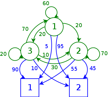
The green part is the Markov chain itself, the blue part corresponds to the observation device. Arcs are labeled with probabilities of transition or observation.

Stepping Forward

Now we can simulate the behavior of the system.

local proba_pick = function(v)
  local p,s = math.random(1,100),0
  for i=1,#v do
    s = s + v[i]
    if p <= s then
      return i
    end
  end
  assert(false)
end

local S,V = {},{}

local transition = function(t)
  assert(S[t-1] and not S[t])
  S[t] = proba_pick(P[S[t-1]])
end

local observe = function(t)
  assert(S[t] and not V[t])
  V[t] = proba_pick(O[S[t]])
end

S[1] = math.random(1,N)
observe(1)

for t=2,L do
  transition(t)
  observe(t)
end

This code is slightly more complicated, but what you should understand is that, at the end of it, S is a vector of L states of the system and V is the corresponding vector of observations. The initial state S[1] is chosen randomly with uniform probabilities.

Seeing Through the Box

Now, let us proceed to guess what happens inside the black box. We do so iteratively: at each tick t, we calculate the most plausible sequence of events that could have led to each possible state of the system, given the observation at t and the results for t-1.

local trellis = {{}}

local prb = function(x)
  return math.log(x/100)
end

local viterbi_node = function(t,i)
  local prev = assert(trellis[t-1])
  local idx,proba = 0,-math.huge
  local p
  for j=1,N do
    p = prev[j].proba + prb(T[j][i]) + prb(1/N*O[i][V[t]])
    if p > proba then proba,idx = p,j end
  end
  return {
    state = i,
    proba = proba,
    prev = prev[idx],
  }
end

local viterbi_step = function(t)
  assert(not trellis[t])
  trellis[t] = {}
  for i=1,N do
    trellis[t][i] = viterbi_node(t,i)
  end
end

-- initialize the trellis
for i=1,N do
  trellis[1][i] = {
    state = i,
    proba = prb(1/N*O[i][V[1]])
  }
end

-- run the algorithm
for t=2,L do
  viterbi_step(t)
end

Again, not trivial code, but this is the Viterbi algorithm itself. Moreover we use logarithmic sums for probabilities to avoid numerical problems.

What the algorithm does is build a trellis, a special kind of graph. For every step t we calculate the most plausible sequence of events (a path through the trellis) which ends up with the system in each of the possible states. When we reach the end of the simulation, we take the most plausible state of the system and take the path that led to it as our estimate of what happened.

To avoid memory usage explosion, we do not actually store the paths themselves in the nodes of the trellis. Instead, in a node at tick t, we store a pointer to the previous node (at t-1) that led there. This is why we have to backtrack through the trellis to find the actual path:

local getpath = function(node)
  local r = {}
  repeat
    table.insert(r,1,node.state)
    node = node.prev
  until (not node)
  return r
end

local best_node = function(nodes)
  local r = {proba = -math.huge}
  for i=1,#nodes do
    if nodes[i].proba > r.proba then
      r = nodes[i]
    end
  end
  return r
end

local bestpath = getpath(best_node(trellis[L]))

Does this thing really work?

To check if this work, let’s take the actual system out of the box and calculate how much it looks like our estimate:

local ok = 0
for i=1,L do
  if S[i] == bestpath[i] then
    ok = ok + 1
  end
end

print(100*ok/L)

The result I got with those parameters is 72% accuracy, to compare to what a naive random process would get (33%).

Why I love it

Let’s go back to the title of this post: now that you know what it does, why is Viterbi’s algorithm my favorite?

I admit that the elegance of the representation of the problem as a trellis is part of the reason, but mainly it’s because of its implications. Think about it: fundamentally it is an algorithm that allows a machine to explain what it observes. Isn’t that crazy?

Yes, it is. And because of that it has a whole range of applications, from advanced orthographic correction and speech-to-text to the decoding of convolutional codes used in voice codecs. And I suspect its potential has not been fully exploited yet.